
JHDL 0.3.39
| JHDL Doc Home Page | User's
Manual Home Page |
The Logic Class: Part 2 - Technology Mapping and Placement
in JHDL
Introduction
What is Mapping and Placement?
"Mapping" is the term used to describe the act of grouping circuitry together
in a primitive FPGA unit. In Xilinx XC4000 parts this primitive block is
the CLB, which includes the mapping of it's constituant LUTs and Registers.
In the Chess architecture, the primitive unit is an ALU or memory block.
What ever the case, mapping groups the specified circuity into a primitive
FPGA block.
Placement is the organizing or arranging of circuits within silicon.
In the context of FPGAs, this involves assigning circuits to a portion
of the gate array. Placement and Mapping will always be done during the
back-end compilation step by automated map, and PAR tools. However, if
for whatever reason a user wishes to customize or optimize how circuitry
is placed or mapped together, manual placement and mapping can be done
during the design entry stage. Placement and Mapping as used in this manual
refer to manual placement and mapping.
Background and Motivation
Placement and Mapping of Circuitry in FPGAs
There are many desirable effects of placement and mapping within FPGAs.
Placement and mapping can:
-
Decrease circuit area
-
Group related logic together in CLBs, ALU, or other primitive unit.
-
Decrease signal delay.
-
This is especially true in FPGAs where routing delay is greater than Circuit
delay.
-
Increase clock frequencies.
-
Preserve regularity
-
Utilize specialized data path features.
-
Standardize Interfaces
-
Decreased compile time
-
This is generally true because the back-end compilation tools are now operating
on Relationally Placed Macros (RPMs) not gates. Of course, my experience
is mostly based on design for Xilinx parts.
Although there are many advantages to manual placement and mapping, it
can be shown that some hybrid solution to placement and mapping between
completely manual and completely automated placement, will produce the
optimum result.
Traditional Placement and Mapping in FPGAs is difficult
Traditionally, Designing for FPGAs was done in VHDL or using a schematic
entry tool like Viewlogic. While Placement in VHDL can be done through
comments, it has many short-comings. Namely that:
-
Structural code and placement comment use different syntaxes.
-
Parameterization is difficult. (this usually requires C code)
-
Very verbose.
-
Long design cycles.
Manual placement can also be done in most schematic entry tools by attaching
property strings to cells. However, this method of design and placement
has many short-comings as well.
-
It is very verbose.
-
Usually offers no programmatic functionality.
-
No parameterization.
-
Long design cycles.
JHDL Technology Mapping and Placement
JHDL was created to address many of difficulties with traditional FPGA
placement and mapping. In particular JHDL
-
Integrates placement code and structural design code in a programmatic
high level language (JAVA).
-
Offers users fine-grained control through the TechMapper.
-
Offers convenience methods for the common cases to reduce verbosity (found
in Logic).
-
Gives designers large amounts of flexibility.
-
Provides Relational placement methods to reduce complexity.
-
Provides Layout Manipulation methods which reduce redesign time.
-
Has error checking done as early as possible.
Logic placement and technology-mapping
In JHDL it is suggested that all designs extend Logic to take advantage
of it's extensive technology independant methods. The Logic class implements
two basic methods for specifying technology-specific placement and mapping:
place()
and
map(). The place method is used to set the relative position
of a cell within the FPGA. Because the Logic API generally returns
Wires
from its cell-instantiating methods, place() will allow the user
to "place" a Wire as well. The inference in this case is that we will place
the cell that drives the given Wire. Thus, we can do the following:
     Wire out = and( a, b );
     place( out, 2, 5 );
allowing us to place the and gate, without ever getting an explicit
handle on the gate itself. The map and place methods in Logic have several
APIs to provide flexibility. Each group of APIs will be explained later
in further detail.
Technology Mapping through Logic
The map() call implies the mapping of a logic function to a target-specific
"atomic cell". The "atomic cell" would be LUTs and flip-flops for the XC4000
architecture, while it would be ALUs and flip-flops for the HP Chess architecture,
etc. The map() call accepts a list of input wires and a single output
wire; this list of wires implies the function that is to be mapped. For
example, if we call:
     Wire out = or( and(a,b), and(a,ci), and(b,ci) );
     map( a, b, ci, out );
this implies mapping the function of the three and gates and one
or
gate into a single LUT or ALU. The map() call currently accepts
from 2 to 9 input parameters, and optionally accepts a String that gives
target-specific constraints to the platform-specific TechMapper.
It is critical to note that the Logic API defines absolutely nothing
about the exact implementation of the map() call, beyond what has
been specified here. The optional String arguments accepted by map()
are specifically "defined to be undefined" in the Logic class! They receive
no interpretation in the Logic class, and are passed straight to the TechMapper
for platform-specific interpretation. Technology mapping can be done explicitly
by instantiaing individual primitives. In the case of a full-adder in XC4000
we would write.
or_o(and(a,b), and(a, ci), and(b, ci), sum);
xor_o(a, b, ci, co);
fmap f1 = new fmap(this, a, b, ci, sum);
fmap f2 = new fmap(this, a, b, ci, co );
However as was mentioned earlier this limits technology independence since
fmaps are specific to Xilinx Parts. The same thing could have been achieved
by targeting the XC4000TechMapper and implementing the fmaps through the
Logic map method. Of course this requires a basic knowledge of Xilinx parts,
to determine how much circuitry will fit into a Look Up Table (LUT) or
CLB. Knowing that a full adder can fit in 2 LUTs or a single CLB. The full
adder with Logic map methods intended for Xilinx XC4000 parts might look
like this:
or_o(and(a,b), and(a, ci), and(b, ci), sum);
xor_o(a, b, ci, co);
map(a, b, ci, sum);
map(a, b, ci, co);
The above map methods will pass all the associated information to the TechMapper.
While some error checking is done in the techmapper,
users are advised to learn the restrictions of a technology before attempting
to use the map method.
Iterated Map
For the convenience of the user, map methods will accept multi-bit wires
and iteratively map the individual bits of the input and output wires.
Again whether a particular group of wires is a valid mapped network depends
on the techmapper being used. If we wanted to map a 5-bit psuedo-adder
we could use the following code in Logic:
Wire a = wire(5);
Wire b = wire(5);
Wire ci = wire(5);
Wire co = wire(5);
Wire sum = wire(5);
or_o(and(a,b), and(a, ci), and(b, ci), sum);
xor_o(a, b, ci, co);
map(a, b, ci, sum);
map(a, b, ci, co);
Each map method in this case would create 5 fmaps or whatever primitive
unit is beign designed for.
Logic Map methods return the new mapping cell or the driver of the
output wire for future use in placement or layout manipulation.
Logic Placement
In general JHDL placement in done by annotating placement hint strings
onto Cells in a netlist. These hints communicate information about where
each cell is to placed to the back-end compilation tools. For example,
Xilinx uses a 2-d array of Logic blocks arranged in Rows and Columns. Each
coordinate in the grid represents a CLB with ".F" ".G", ".H", ".FFX", and
".FFY" representing the associated parts of the CLB.
"Hints", or properties may be specified in many different ways. The
most primitive method, which allows users very fine-grained control with
out JHDL intervention, is to use the addProperty() method.
To place the 1-bit full adder of the previous example in XC4000
we could use the following code:
or_o(and(a,b), and(a, ci), and(b, ci), sum);
xor_o(a, b, ci, co);
map(a, b, ci, sum).addProperty("RLOC", "R0C0.F");
map(a, b, ci, co).addProperty("RLOC", "R0C0.G");
This will append the property string "RLOC=R0C0.F" onto the fmap returned
by the map method for the sum circuitry, and append the property
string "RLOC=R0C0.G" onto the fmap for the carry circuitry.
The place method in Logic is designed to be a convenient way
of appending placement hints onto a cell. Placement hints can be entered
directly into the place method without the
RLOC String
like so....
place(Cell Sum, "R0C0.F");
place(Cell Carry, "R0C0.G");
These simple place methods will simply attach an RLOC property with the
given value to the specified Cells.
In order to preserve some notion of technology independence when placing,
a generic grid of X and Y coordinates is used in Logic and interpreted
by each TechMapper. Then at netlist time these X and Y coordinates with
any hints are converted into properties like the RLOCs for XC4000 and attached
to the appropriate cells. The JHDL placement grid allows Logic to do some
conversion of hints before Technology Mapping and to determine if a cell
is placeable according to the given techmapper. It also allows the use
of ints instead of Strings, which improves programmatic functionality.
The technology still determines which placement hints are valid. The conversion
from a JHDL placement grid to XC4000 and Virtex is illustrated below.
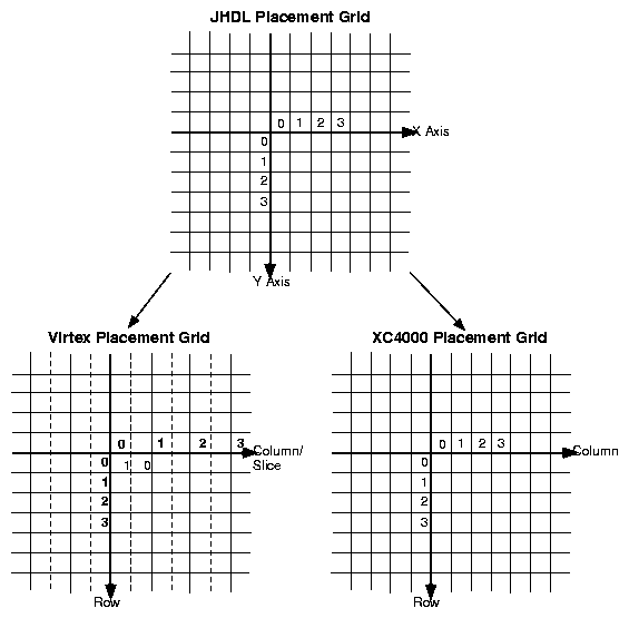
Placement Standards
In order to eliminate confusion, reduce complexity, and catch more errors,
several placement standards exist within JHDL. They are:
-
The location of the placement origin is fixed at the upper-left corner
of a cell's bounding box. The bounding box is computed just before placing
a cell, thus allowing consistent notation and knowledge of what is being
placed, width, and heights of cells.
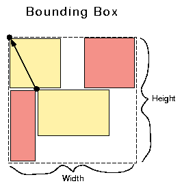
-
The placement of a cell's children may not be changed once it is placed,
unless the layout is transformed in a predefined manner. This is referred
to as a locked placement and it prevents circumvention of placement
checking and computation of bounding box.
-
Multi-level library cells have a standard layout in each technology.
-
In Xilinx libraries this standard is to have cells laid out in:
-
Vertical columns
-
LSB on bottom, MSB on top
-
Data flow from left to right
Positional Placement
Positional placement is the term used for placing a cell at a certain numerical
location withing a layer of hierarchy. In JHDL this is done on a two-dimensional
grid of X and Y coordinates.
Placement in this fashion can be done in the following way for the Full-Adder
example in XC4000.
or_o(and(a,b), and(a, ci), and(b, ci), sum);
xor_o(a, b, ci, co);
map(a, b, ci, sum);
place(sum, 0, 0, ".F");
map(a, b, ci, co);
place(co, 0, 0, ".G");
This code will place the sum logic at X=0 Y=0 with a ".F" String property
that will be passed to the TechMapper of choice and interpreted there.
The same will be true of the carry logic except it will have the ".G" String.
We could have placed the two pieces of circuitry at any position within
this layer of hierarchy, however, recall that placement is always done
by the upper left hand corner of the bounding box. Therefore, these locations
are only valid within this layer of hierarchy. Another, less effiecient
placement of the circuit would look like this.
or_o(and(a,b), and(a, ci), and(b, ci), sum);
xor_o(a, b, ci, co);
map(a, b, ci, sum);
place(sum, -1, -1, ".F");
map(a, b, ci, co);
place(co, 1, 2, ".G");
In this case the two circuits are placed at X=-1 Y=-1 and X=1, Y=2 repectively.
Relational Cell Placement
"Relational cell placement" is the term used to describe the ability to
place a cell based on width, height, or location of this cell and/or another.
It was created to simplify many common placement cases. In particular it
is intended to:
-
Reduce the complexity of numerical calculations for placement
-
Increase technology independence among designs
-
Improve readability and reduce verbosity
Relational Cell Placement is done by using information about Cells to compute
a new placement location. This information includes the width and height
of cells, and the placement location of cells. This information ( X, Y,
Width, Height ) is stored in each Cell and can be accessed through methods
on cell. These methods are
getX()
getY()
getWidth()
getHeight()
By themselves these methods do not accomplish much, but with convenience
methods that used them they can be very powerful tools. These convenience
methods are implemented in Logic and accept Cells or output Wires as usual.
The basic format for relational cell placement is
Place(Cell curr, Directive dir, Cell prev);
Just as if reading a sentence this method would place the current cell
in the direction of dir from a previous cell. For example, absolute placement
of a registered adder might look something like this:
Wire sum = add(a,b);
Wire out = reg(sum);
place(sum, 0, 0);
place(out, 1, 0);
However, the same basic placement could be achieved with relational
placement in the following way:
Wire sum = add(a,b);
Wire out = reg(sum);
place(out, RIGHT_OF, sum);
Notice that the relational placement does not require knowledge about
the width of the register or the adder. These methods can be simply read
as "place the register to the right of the adder". The relational methods
in Logic will decide where the register should be placed based on the specified
direction.
Directives
Direction is specifed with the Directive object. 10 Static Directive objects
have been created in Logic to handle the common cases. These ten all follow
two basic naming schemes as shown in table 1 and figure 1 below.
Table 3.1: Directives in Logic
| Naming |
Naming |
Direction |
| Scheme 1 |
Scheme 2 |
|
| ABOVE |
NORTH_OF |
UP |
| BELOW |
SOUTH_OF |
DOWN |
| RIGHT_OF |
EAST_OF |
TORIGHT |
| LEFT_OF |
WEST_OF |
TOLEFT |
| ON |
ONTOP_OF |
ONTOP |
|
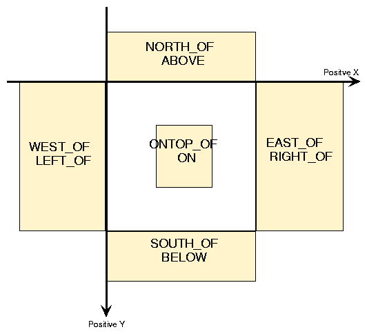 |
Figure 1New Placement Directives
on JHDL Grid
When a relational placement method like the one below is used, several
steps are followed to place Cell1.
place(Cell1, Directive, Cell2);
-
Compute the bounding box of Cell2 if unknown.
-
Place Cell2 at X=0, Y=0 if it is unplaced.
-
Compute bounding box of Cell1.
-
Compute placement location for Cell1 from widths, heights, X, Y, and Directive.
-
Place Cell1 and Lock it's placement.
NOTE: Order is important! Remember that if in the above example, Cell2
was previously unplaced, and place(Cell3, Directive, Cell4); is
called with Cell4 not already placed, Cell4 will be placed at X=0, Y=0,
which is ON TOP of Cell2, probably not what you want. To avoid this, place
Cell4 relative to Cell1 or Cell2 first.
Alignment with Directives
All directives have two optional alignment fields. Vertical alignment,
which can be used when placing horizontally or in the X direction,
and horizontal alignment, which can be used when placing vertically or
in the Y direction. When placing a cell on top of another cell,
both alignment fields will be used since neither the X nor the Y
direction is being specified. Each of the two alignment fields can have
any one of three values.
In order to specify which type of alignment is to be used when placing,
methods are provided in the Directive class. These methods can be used
on the Directives in the place call like so:
place( CellA, RIGHT_OF.alignTop(), CellB);
The above method would thus read, place CellA to the
right of
CellB such that top edges are aligned. If Directives
are used without these alignment methods, then the default will be to align
left edges, top edges, or both. There are several different methods for
changing or setting the alignments of a Directive. They are:
Alignment Methods on Directives
-
Vertical Alignment
-
.alignTop()
-
.alignBottom()
-
Horizontal Alignment
-
.alignLeft()
-
.alignRight()
-
Both
Examples, of each alignment are shown for each Directive below.
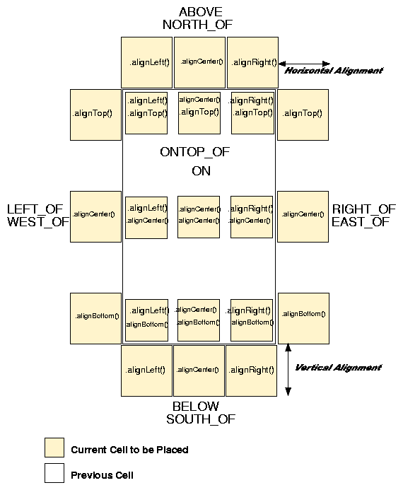 |
Figure 2:New Placement Directives
and Alignments
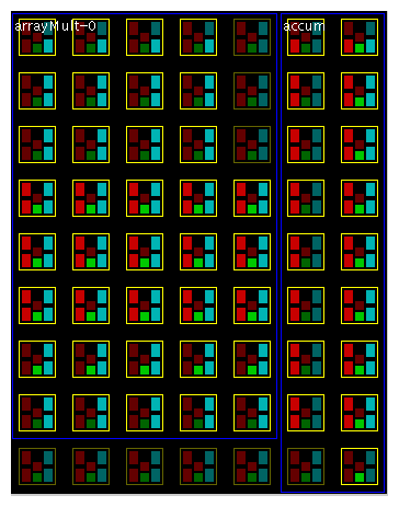
Multiply Accumulate Example
As an example, consider the design of a multiply accumulate of variable
width and length. If we wanted to place the accumulator to the right of
the multiplier, no matter what it's dimensions are we could us relational
placement like so:
Cell multiplier = new arrayMult(this, OperandA, OperandB, vcc(), Product, signed, fully_pipelined);
place(multiplier, 0, 0);

Cell accumulator = new accum(this, Product, gnd(), vcc(), vcc(), Total);
place(accumulator, RIGHT_OF, multiplier);
The result would look something like this in the XC4000 Layout viewer.
Cell Transformations
Cell transformations is the name given to a group of methods in Logic that
change a Cell's layout or placement while preserving functionality. Cell
transformations provide users with different layouts while preserving connectivity
of a cell or module. They allow users to change data-flow direction, wrap
linear data paths, match port pitch, and move relative to other cells.
Currently, 3 transformations exist: scale, rotate, and
translate
.
They are all methods in the logic class and will accept either cells or
output wires.
Scale
scale(cell C, int xFact, int yFact);
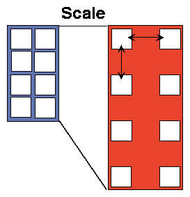
The scale method is designed to stretch a cell's layout by xFact
in the x direction and yFact in the y direction. It works by recursively
moving children cells to the new position x = x*xFact, y = y*yFact and
then recomputing the cell's bounding box. This scaling of the layout can
only be done before a cell is placed.
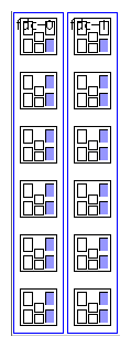
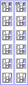
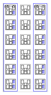
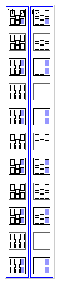
Example 2
Wire d = wire(11);
Wire q = wire(11);
Cell regbank = new regBank(this, d, q);
scale(regbank, 1, -1);
place(regbank, 0, 0);
These figures show the original register bank, scaled by -1 in Y, scaled
by 2 in X, and scaled by 2 in Y.
LIMITATIONS
Currently, the scale method only accepts Integer factors. Great care should
also be taken to ensure that Asymmetric features of the FPGA are not scaled,
as this will cause an error in the back-end compilation.
Rotate
rotate(cell C, int deg);
The rotate method rotates a Cell's layout by deg degrees
in a counter-clockwise direction. It is implemented by recursively moving
children to a new position, and then recomputing each cell's bounding box.
Again the rotate method is only valid on a cell that has not yet been placed.
It also has many of the same limitations as scale.
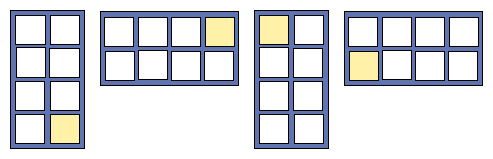
ROTATION by 0, 90, 180, 270
Example 3
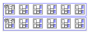
As an example let's say we wanted to rotate the previous register bank
by 90 degrees in the counter-clockwise direction. We could use:
Wire d = wire(11);
Wire q = wire(11);
Cell regbank = new regBank(this, d, q);
rotate(regbank, 90);
place(regbank, 0, 0);
The result would look like this in XC4000.
Translate
translate(cell C, int dx, int dy);
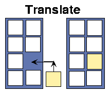
The translate method allows users to move a Cell by dx and dy
from it current position. It has the exact same effect as using
place(x+dx,
y+dy); where x and y are the cell's current placement position. Unlike
scale
and rotate,
translate can only be used after a cell is placed.
Example 4
Assume that there is a known hole in a module as shown in the fiugre above.
The translate method could be used to fill that hole with a register as
shown through the code below.
new Mod1(this, in1, in2, out);
Wire delay = reg(out);
place(Mod1, 0, 0);
place(delay, RIGHT_OF.alignBottom(), out);
translate(delay, -1, -1);
Relational Port Placement
As we have seen thus far relational cell placement can be very useful for
minimizing the FPGA area consumed by a design. Relational Port Placement
is designed to minimize delay through the circuitry by aligning ports,
or wires.
Verbose Port Placement Method
place(Cell currcell, Wire inWire, Directive dir, Cell prevcell, Wire
outWire);
This is the most verbose method for relational port placement. It directs
Logic to place currcell in the direction of
dir from
prevcell,
aligning
inWire and outWire.
The steps to doing this relational port placement are as follows.
-
Find port location in prevcell.
-
Find the leaf cell associated with the alignment wire (source) and ignore
cells that cannot be placed.
-
Compute it's absolute location within the parent.
-
Find port location in currcell.
-
Place relationally aligning port locations.
Convenience Methods
place(cell1, dir.align(Wire), cell2);
To eliminate most of the verbosity of the relational port placement
method, relational port placement can be done through the relational cell
placement methods. This is done by using alignment methods on the Directive
which specify the wire to align the two cells with.
To illustrate consider the placement of a registered adder.
Wire sum = add(a,b);
Wire out = reg(sum);
place(out, ONTOP_OF.align(sum), sum);
The above code segment would place the adder at X=0, Y=0 and then place
the register in the same location as the adder so that the sum wire fed
directly out of the adder and into the register.
Port Placement and Alignment
Since Multi-bit ports with different pitch cannot be perfectly aligned
without using the scale method, Alignment methods on Directives were created
to specify which bit of the port wire to align. These methods are:
-
.alignCenter(Wire w) [default]
-
.alignLSB(Wire w)
-
.alignMSB(Wire w)
Summary
-
JHDL Placement reduces complexity.
-
Low level designs are easier to place.
-
Parameterized placement of modules is much easier.
-
Placement of large designs is now feasible.
-
JHDL Placement improves readability and eliminates verbosity.
-
Most JHDL Placement can be shared across technologies.
-
Convenience methods and error checking reduces design time.
-
Designers can spend more time finding an optimum layout and mapping, without
dwelling on the semantics of the language.
-
Iteration on a designs technology mapping and placment is now possible.
| JHDL Doc Home Page | User's
Manual Home Page |

Copyright (c) 1998-2003 Brigham Young University. All rights reserved.
Reproduction in whole or in part in any form or medium without express
permission of Brigham Young University is prohibited.
Documentation Revision: 19 Mar, 2001